Introduction

In this part, I’ll walk you through a practical example about how to handle missing data using a dataset with missing values. I will show different imputation techniques and discuss their impacts.

Practical Examples

Let’s walk through a practical example using a dataset with missing values. We will demonstrate different imputation techniques and discuss their impacts.

Example: Handle Missing Data in the Titanic dataset

I will now demonstrate different imputation techniques using the Titanic dataset, which includes missing values in columns like Age and Embarked.

import pandas as pd
import seaborn as sns
from sklearn.impute import SimpleImputer, KNNImputer
from sklearn.experimental import enable_iterative_imputer
from sklearn.impute import IterativeImputer
from sklearn.model_selection import train_test_split

# Load the Titanic dataset
df = sns.load_dataset('titanic')

Now let’s have a look at the top 5 the rows of the dataframe:

df.head(5)

survived	pclass	sex	age	sibsp	parch	fare	embarked	class	who	adult_male	deck	embark_town	alive	alone
0	3	male	22.0	1	0	2,027777778	S	Third	man	TRUE	NaN	Southampton	no	FALSE
1	1	female	38.0	1	0	4,925694444	C	First	woman	FALSE	C	Cherbourg	yes	FALSE
1	3	female	26.0	0	0	6,715277778	S	Third	woman	FALSE	NaN	Southampton	yes	TRUE
1	1	female	35.0	1	0	2,902777778	S	First	woman	FALSE	C	Southampton	yes	FALSE
0	3	male	35.0	0	0	0,6805555556	S	Third	man	TRUE	NaN	Southampton	no	TRUE

Checking Missing Data

Let’s check for missing data:

df.isnull().sum()

which gives:

survived         0
pclass           0
sex              0
age            177
sibsp            0
parch            0
fare             0
embarked         2
class            0
who              0
adult_male       0
deck           688
embark_town      2
alive            0
alone            0
dtype: int64

Then, let’s split the dataset into training and test set:

# Select features and target variable
features = ['pclass', 'sex', 'age', 'sibsp', 'parch', 'fare', 'embarked']
target = 'survived'

# Convert categorical features to numeric
df['sex'] = df['sex'].map({'male': 0, 'female': 1})
df['embarked'] = df['embarked'].map({'C': 0, 'Q': 1, 'S': 2})

# Split the dataset
X = df[features]
y = df[target]
X_train, X_test, y_train, y_test = train_test_split(X, y, test_size=0.2, random_state=42)

# Display the shape of the resulting datasets
print(f'Training set shape: {X_train.shape}')
print(f'Testing set shape: {X_test.shape}')

Which will output:

>>> Training set shape: (712, 7)
>>> Testing set shape: (179, 7)

Imputing The Missing Data

Now, we will apply all the different missing imputation techniques

# Mean Imputation for 'Age'
mean_imputer = SimpleImputer(strategy='mean')
X_train['age_mean'] = mean_imputer.fit_transform(X_train[['age']])
X_test['age_mean'] = mean_imputer.transform(X_test[['age']])

# Median Imputation for 'Age'
median_imputer = SimpleImputer(strategy='median')
X_train['age_median'] = median_imputer.fit_transform(X_train[['age']])
X_test['age_median'] = median_imputer.transform(X_test[['age']])

# KNN Imputation for 'Age' and 'Fare'
knn_imputer = KNNImputer(n_neighbors=5)
X_train[['age_knn', 'fare_knn']] = knn_imputer.fit_transform(X_train[['age', 'fare']])
X_test[['age_knn', 'fare_knn']] = knn_imputer.transform(X_test[['age', 'fare']])

# MICE Imputation for 'Age'
mice_imputer = IterativeImputer()
X_train['age_mice'] = mice_imputer.fit_transform(X_train[['age']])
X_test['age_mice'] = mice_imputer.transform(X_test[['age']])

Now, let’s compare all the various results:

import matplotlib.pyplot as plt
import seaborn as sns

# Plot the original and imputed 'Age' distributions
plt.figure(figsize=(12, 6))
sns.kdeplot(df['age'], label='Original Age', color='blue', fill=True)
sns.kdeplot(df['Age_mean'], label='Mean Imputed Age', color='red', linestyle='--', fill=True)
sns.kdeplot(df['Age_knn'], label='KNN Imputed Age', color='green', linestyle='--', fill=True)
sns.kdeplot(df['Age_mice'], label='MICE Imputed Age', color='purple', linestyle='--', fill=True)
plt.legend()
plt.title('Comparison of Age Distributions After Imputation')
plt.show()

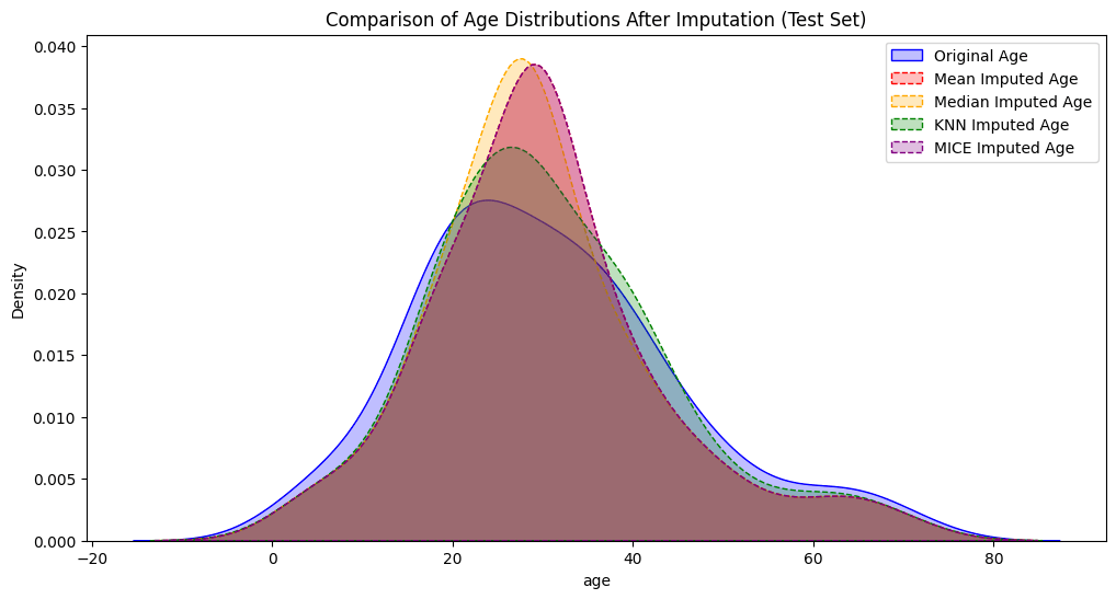
As it’s possible to see on the chart, it looks like that in this case the KNN imputer is the one which is closer to the distribution of the original variable age to be imputed.

Food for Thoughts

To handle missing data is a critical skill for data scientists. Understanding the advantages and limitations of each method helps in making informed decisions. During interviews, knowing these techniques can make a candidate stand out. It shows their expertise in data prep and model building.

Use these methods well. They will keep your data safe and your models reliable.

If you liked this article, you might also like this one about How to Choose the Best Categorical Encoding Method

Let’s Connect

You can also find me on:

• X/Twitter: @feddernico
• Medium: @federico.viscioletti
• Substack: https://feddernico.substack.com/